Before we begin, I'd like to point out that object placed around the antenna will alter its radiation pattern. As a result, its input impedance will be influenced by what is around it - i.e. the environment in which the antenna is tested. Consequently, for the best accuracy the impedance should be measured in an environment that will most closely resemble where it is intended to operate. For instance, if a blade antenna (which is basically a dipole shaped like a paddle) is to be utilized on the top of a fuselage of an aiprlane, the test measurement should be performed on top of a cylinder type metallic object for maximum accuracy. The term driving point impedance is the input impedance measured in a particular environment, and self-impedance is the impedance of an antenna in free space, with no objects around to alter its radiation pattern.

Fortunately, impedance measurements are pretty easy if you have the right equipment. In this case, the right equipment is a Vector Network Analyzer (VNA). This is a measuring tool that can be used to measure the input impedance as a function of frequency. Alternatively, it can plot S11 (return loss), and the VSWR, both of which are frequency-dependent functions of the antenna impedance. The Agilent 8510 Vector Network Analyzer is shown in Figure 1.

 

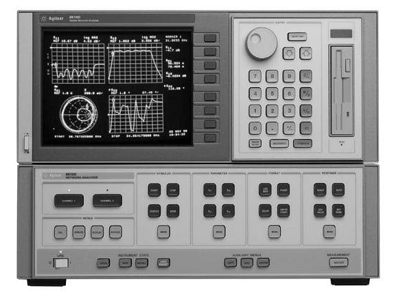
Figure 1. The popular Agilent (HP) 8510 VNA.

Let's say we want to perform an impedance measurement from 400-500 MHz. Step 1 is to make sure that our VNA is specified to work over this frequency range. Network Analyzerswork over specified frequency ranges, which go into the low MHz range (30 MHz or so) and up into the high GigaHertz range (110 GHz or so, depending on how expensive it is). Once we know our network analyzer is suitable, we can move on.

Next, we need to calibrate the VNA. This is much simpler than it sounds. We will take the cables that we are using for probes (that connect the VNA to the antenna) and follow a simple procedure so that the effect of the cables (which act as transmission lines) is calibrated out. To do this, typically your VNA will be supplied with a "cal kit" which contains a matched load (50 Ohms), an open circuit load and a short circuit load. We look on our VNA and scroll through the menus till we find a calibration button, and then do what it says. It will ask you to apply the supplied loads to the end of your cables, and it will record data so that it knows what to expect with your cables. You will apply the 3 loads as it tells you, and then your done. Its pretty simple, you don't even need to know what you're doing, just follow the VNA's instructions, and it will handle all the calculations.

Now, connect the VNA to the antenna under test. Set the frequency range you are interested in on the VNA. If you don't know how, just mess around with it till you figure it out, there are only so many buttons and you can't really screw anything up.

If you request output as an S-parameter (S11), then you are measuring the return loss. In this case, the VNA transmits a small amount of power to your antenna and measures how much power is reflected back to the VNA. A sample result (from the slotted waveguides page) might look something like:

 

Figure 2. Example S11 measurement.

Note that the S-parameter is basically the magnitude of the reflection coefficient, which depends on the antenna impedance as well as the impedance of the VNA, which is typically 50 Ohms. So this measurement typically measures how close to 50 Ohms the antenna impedance is.

 

Another popular output is for the impedance to be measured on a Smith Chart. A Smith Chart is basically a graphical way of viewing input impedance (or reflection coefficient) that is easy to read. The center of the Smith Chart represented zero reflection coefficient, so that the antenna is perfectly matched to the VNA. The perimeter of the Smith Chart represents a reflection coefficient with a magnitude of 1 (all power reflected), indicating that the antenna is very poorly matched to the VNA. The magnitude of the reflection coefficient (which should be small for an antenna to receive or transmit properly) depends on how far from the center of the Smith Chart you are. As an example, consider Figure 3. The reflection coefficient is measured across a frequency range and plotted on a Smith Chart.

 

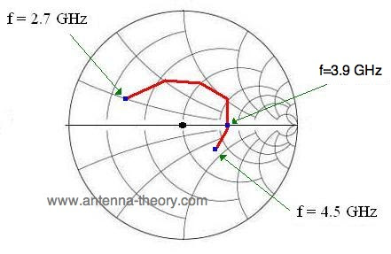
Figure 3. Smith Chart Graph of Impedance Measurement versus Frequency.

In Figure 3, the black circular graph is the Smith Chart. The black dot at the center of the Smith Chart is the point at which there would be zero reflection coefficient, so that the antenna's impedance is perfectly matched to the generator or receiver. The red curved line is the measurement. This is the impedance of the antenna, as the frequency is scanned from 2.7 GHz to 4.5 GHz. Each point on the line represents the impedance at a particular frequency. Points above the equator of the Smith Chart represent impedances that are inductive - they have a positive reactance (imaginary part). Points below the equator of the Smith Chart represent impedances that are capacitive - they have a negative reactance (for instance, the impedance would be something like Z = R - jX).

To further explain Figure 3, the blue dot below the equator in Figure 3 represents the impedance at f=4.5 GHz. The distance from the origin is the reflection coefficient, which can be estimated to have a magnitude of about 0.25 since the dot is 25% of the way from the origin to the outer perimeter.

As the frequency is decreased, the impedance changes. At f = 3.9 GHz, we have the second blue dot on the impedance measurement. At this point, the antenna is resonant, which means the impedance is entirely real. The frequency is scanned down until f=2.7 GHz, producing the locus of points (the red curve) that represents the antenna impedance over the frequency range. At f = 2.7 GHz, the impedance is inductive, and the reflection coefficient is about 0.65, since it is closer to the perimeter of the Smith Chart than to the center.

In summary, the Smith Chart is a useful tool for viewing impedance over a frequency range in a concise, clear form.

Finally, the magnitude of the impedance could also be measured by measuring the VSWR (Voltage Standing Wave Ratio). The VSWR is a function of the magnitude of the reflection coefficient, so no phase information is obtained about the impedance (relative value of reactance divided by resistance). However, VSWR gives a quick way of estimated how much power is reflected by an antenna. Consequently, in antenna data sheets, VSWR is often specified, as in "VSWR: < 3:1 from 100-200 MHz". Using the formula for the VSWR, you can figure out that this menas that less than half the power is reflected from the antenna over the specified frequency range.

In summary, there are a bunch of ways to measure impedance, and a lot are a function of reflected power from the antenna. We care about the impedance of an antenna so that we can properly transfer the power to the antenna.

In the next Section, we'll look at scale model measurements.